Viper examples

• Here you will find downloadable setup files for computing several example flows using Viper. These test cases take only minutes to complete on a single CPU core.

  Each package contains a mesh file (e.g. mesh01.msh), Viper configuration file viper.cfg and a text file containing a list of commands to be executed by Viper (e.g. macro.txt). The Viper Reference Manual should be consulted for explanations of Viper's mesh format, configuration file and available commands, some of which appear in the examples on this page.

  Linux

  We recommend placing the Viper executable in a folder, and each set of downloaded setup files in separate subfolders. From a subfolder, invoke the code using ../viper.x < macro.txt, where the "<" directs Viper to take input from the text file macro.txt rather than the keyboard.

  Windows

  Place a copy of the Viper executable and each set of downloaded setup files in separate folders. From one of these folders invoke the Viper executable, then on the Viper command line enter macro macro.txt to parse the contents of the macro.txt file.

  Visualization

  Viper can output binary .plt data files, readable by Tecplot 360, for visualization of instantaneous flow solutions.

Lid driven cavity

• 2D solver (Cartesian coordinates)

  

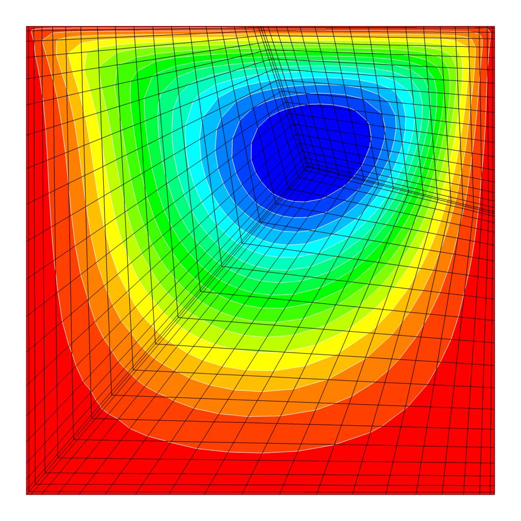  Steady state lid driven cavity flow solution at Re = 100. The top boundary has a constant velocity to the right, contours show the streamfunction, and the mesh (including interpolation points within elements) is overlaid.

  The flow within a two-dimensional square cavity driven by a constant horizontal velocity at the top boundary, the classical lid driven cavity flow, is a ubiquitous benchmark problem for Navier-Stokes solvers in computational fluid dynamics. The test case provided here (download: .tgz or .zip) demonstrates Viper's solution of this problem for a Reynolds number (based on the lid velocity and cavity side length) Re = 100, evolving the flow to its steady state from a quiescent initial condition.

  For demonstration purposes, the mesh used in this example has three irregularly shaped elements, each having 20 × 20 interpolation points. Despite this modest resolution, the steady-state solution compares well to benchmark results from Botella & Peyret (1998). The minimum velocity on the vertical enclosure centreline is -0.212 (compared with their -0.214), the minimum and maximum vertical velocities on the horizontal centreline are -0.215 (-0.214) and 0.178 (0.179), and the vorticity at the centre point is -1.16 (-1.17). Note: the Botella & Peyret values are opposite-signed in their tables 2 and 3 as their lid velocity was right-to-left rather than the left-to-right adopted here.

  The macro commands first set the time step (init), then execute 12 blocks of 1000 time steps (the loop-step-endl part), before finally outputting data from the simulation. Two line commands output the min/max data along the horizontal and vertical centrelines, sample is used to extract data at the centre point of the domain, and tecp outputs a Tecplot file for visualisation.

  Exercises

  Try varying the order of the elements (the gvar_N parameter in the viper.cfg file specifies the number of interpolation points in each direction within each element). Coarser solutions are obtained at smaller values.

  Try varying the Reynolds number (the gvar_RKV parameter in the viper.cfg file here is equivalent to the Reynolds number).

  Try varying the time step (using the set dt command in the macro file. You will find the time integration becomes unstable beyond some time step. The stability and accuracy of the 3rd-order backwards differentiation time integration scheme employed by Viper is described in Karniadakis, Israeli & Orszag (1991).

  Related examples

  The discontinuities at the domain corners where the moving lid meets the stationary side-walls degrade the convergence of the solutions. An alternative is to adopt a regularised lid boundary condition expressed as a function whose value and gradient are both zero at the corners. Peyret & Taylor (Computational Methods for Fluid Flow, Springer, 2012) present a lid velocity u(x) = 16x²(1-x²), which is adopted here (download: .tgz or .zip) on the same three-element mesh.

  Also included is a further example comprising a 25-element mesh (featuring 5 by 5 elements with compression near each of the four boundaries; download: .tgz or .zip). The larger number of elements means that a lower element polynomial order can achieve a similar resolution to higher-order simulations in the previous example case. Conversely, this example case solves the same problem on a single-element mesh (download: .tgz or .zip).

Flow past a sphere

• Axisymmetric solver (cylindrical coordinates)

  

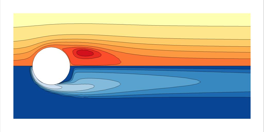  Steady state axisymmetric flow past a sphere at Re = 200. Flow is left to right, and contours show the streamfunction (top) and vorticity (bottom).

  The flow past a sphere is a canonical bluff-body flow problem. In Viper's cylindrical solver, horizontal and vertical mesh coordinates respectively correspond to the axial (z) and radial (r coordinates. The solver automatically imposes the required boundary conditions on the axis (r = 0), so no boundary conditions need to be explicitly defined there. It is also not sensible to have any part of the domain extend to negative r values. This test case (download: .tgz or .zip) comprises a 385-element mesh having 6-by-6 interpolation points per element. The Reynolds number based on the freestream velocity and sphere diameter is Re = 200.

  This example case uses the gvar_curve command in the viper.cfg file to apply curvature to the sphere surface. The axi command in the macro.txt file invokes the cylindrical solver, while the forces command computes the force due to pressure and viscous shear acting on the sphere. Under this non-dimensionalisation, conversion of the axial force to a drag coefficient requires division by π/8. This case achieves a drag coefficient C_d = 0.771. For comparison, the computations by Natarajan & Acrivos (1993) yielded C_d = 0.78, though in a domain with greater radial confinement.

  Exercises

  Try varying the Reynolds number. In this case too, the gvar_RKV parameter in the viper.cfg file is equivalent to the Reynolds number. How do your computed drag coefficients compare to those in Sheard et al. (2005)?

Confined swirling flow

• Axisymmetric solver with swirl (cylindrical coordinates)

  

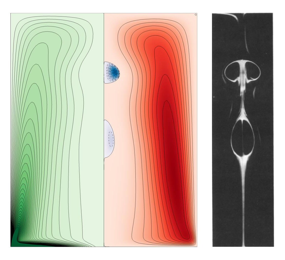  Confined swirling flow solution at Re = 200 and H/R = 2.5. The bottom boundary is rotating. Left and right halves show contours of angular momentum and stream function, respectively. To the right is a dye visualization obtained at the same conditions by Escudier (1984) for comparison.

  This example case (download: .tgz or .zip) computes the flow in a closed fluid-filled cylindrical container driven by rotation of one end-wall. This system produces vortex breakdown beyond a critical Reynolds number. Here Re = 2126 is solved, based on the cylinder radius and end-wall angular velocity, exhibiting two vortex breakdown bubbles at saturation (e.g. see Escudier 1984; Lopez 1990).

  Exercises

  Try varying the Reynolds number to reproduce other flow states from Escudier (1984) or Lopez (1990), such as the bubble merger between Re = 2.1 × 10³ and 2.5 × 10³, or the absence of bubbles below Re < 1.9 × 10³.

Flow past a circular cylinder

• 2D solver (Cartesian coordinates)

  

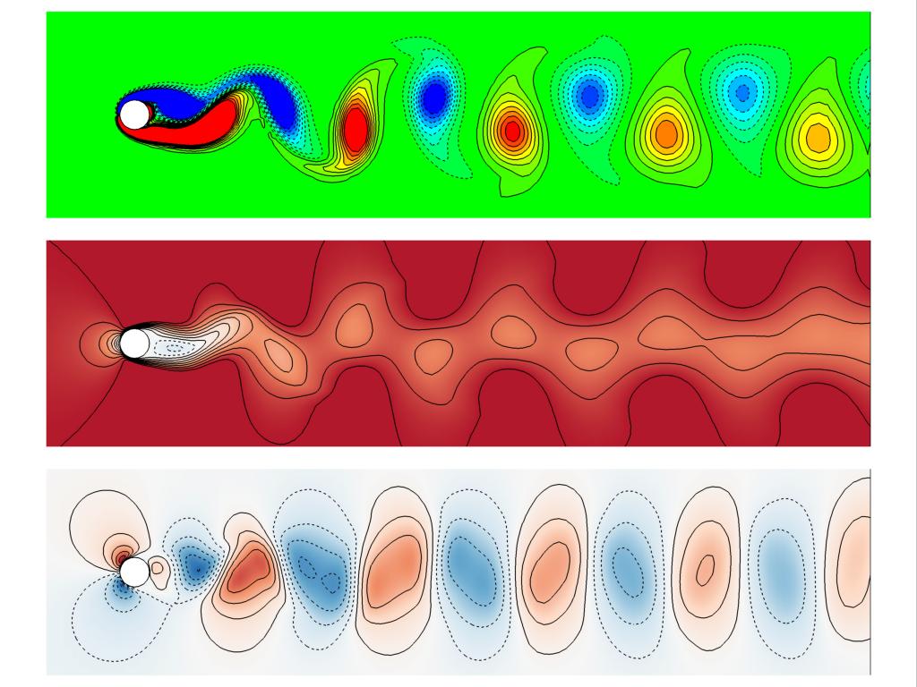  The classical von Kármán vortex street behind a circular cylinder, at Re = 100. Top, middle and bottom frames show vorticity, u- and v-velocity components, respectively.

  In contrast to the earlier cases, this example (download: .tgz or .zip) computes the flow past a circular cylinder at a Reynolds number (based on cylinder diameter and freestream flow speed) Re = 100. This flow is unstable to a time-dependent 2D instability that produces the Kármán vortex street, comprising a periodic shedding of positively- and negatively-signed vortices from alternating sides of the cylinder, which then convect downstream. This case includes the command rand, that adds a small random perturbation to the flow field. This encourages the growth of the instability captured in this simulation, reducing the required compute time.

  Exercises

  The instability producing the Kármán vortex street is absent below Re ≈ 47. Try simulating the flow at a lower Reynolds number (e.g. Re = 40): what does the steady-state wake look like? How does it compare to the wake behind a sphere from the earlier example case?

  The supplied macro file outputs a domain integral (the int command) of the square of the velocity perturbation (local velocity minus freestream velocity), and the forces on the cylinder. Try plotting the total vertical (y-direction) force time history. You should see an oscillatory response that grows exponentially, before saturating to a constant-amplitude time-periodic state. Interpolate to find the times at which the oscillation increases through zero. This time period should be close to 5.997668. Under the non-dimensionalisation adopted here, the Strouhal number is simply the reciprocal of this dimensionless time period, i.e. St = 1/5.997668 = 0.1667. The universal St-Re curve fit developed by Williamson (1988) from experimental data yields a similar St = 0.164.

  Animation sequences

  The time-periodic von Kármán vortex street behind a circular cylinder at Re = 100.

  In this example (download: .tgz or .zip), the Viper restart file generated by the previous example case (save_circ_cyl_2d_re100.dat) is loaded as an initial condition for a run designed to save 64 equi-spaced snapshots of the flow over precisely one shedding period for animation. This is facilitated by first modifying the time step size so that 64 blocks of 19 time steps are integrated, with a Tecplot file saved each time. The "-s" option is used in the tecp call to save a numbered sequence of Tecplot files for later visualization and animation.

  Lagrangian passive tracer particles

  Simulating planar laser induced fluorescent dye visualization of the 2D flow past a circular cylinder at Re = 100. Viper's high-order Lagrangian passive tracer particle evolution capability is employed, with 64 particles injected into the flow from a circle 0.05 diameters from the cylinder surface every 5 time steps.

  Viper implements a high-order time integration scheme for passive tracer particles, exploiting the full resolution of the spectral elements. The scheme was proposed by Coppola, Sherwin & Peiró (2001). This example (download: .tgz or .zip), demonstrates how Viper can be set up to carry out a passive tracer particle transport on a time varying flow field - here the time-periodic flow past a circular cylinder at Re = 100. In this example, 64 particle injectors are equi-spaced around a circle 0.05 diameters above the cylinder surface, and particles are injected every 5 time steps into the flow. By the end of the displayed animation, approximately 100,000 particles are in the flow. This setup closely mimics classic electrolytic precipitation or fluorescent dye visualization experiments used to visualize the Kármán vortex street (e.g. see Milton van Dyke's excellent An Album of Fluid Motion).

  This passive tracer particle transport capability is also implemented in Viper's spectral element-Fourier 3D solver. Sheard et al. (2009) used this feature to demonstrate the three-dimensional wake modes behind an inclined square cylinder, including the elusive subharmonic "Mode C" instability mode.

  Linear stability analysis

  The 3D linear mode A instability in the wake of the cylinder at Re = 189.

  In this example (download: .tgz or .zip), a linear stability analysis is demonstrated. In Viper, the linear stability analysis capability determines the stability of a two-dimensional base flow to two- or three-dimensional infinitesimal perturbations. This example captures the first three-dimensional instability in the wake of a circular cylinder at Re = 189, having a spanwise periodic structure with wavelength of 3.96 diameters. This is consistent with the pioneering analysis of Barkley & Henderson (1996).

  This example is packaged with three macro files. First, macro_2d.txt should be run, which time integrates the two-dimensional flow sufficient to reach a time periodic state. This serves as the initial condition and base flow for the linear stability analysis. Secondly, macro_lsa.txt is used to perform the analysis. In this macro file the pert command activates a linearised three-dimensional perturbation field with spanwise wavenumber 1.585, and the command lsa is a driver routine that conducts the stability analysis. The analysis iterates until the requested leading eigenmode is found. The eigenvalue magnitude reveals the stability (> 1 being unstable; < 1 being stable): here the magnitude should be a weakly unstable 1.0053, consistent with Barkley & Henderson's predicted critical Reynolds number Re_c = 188.5. Finally, macro_3d_vizmode.txt uses Viper's spectral element-Fourier 3D capability to superpose the 2D base flow and three-dimensional perturbation, outputting the result to a three-dimensional Tecplot file for visualization.

Natural convection in a square cavity

• Boussinesq natural convection with differentially heated side walls

  

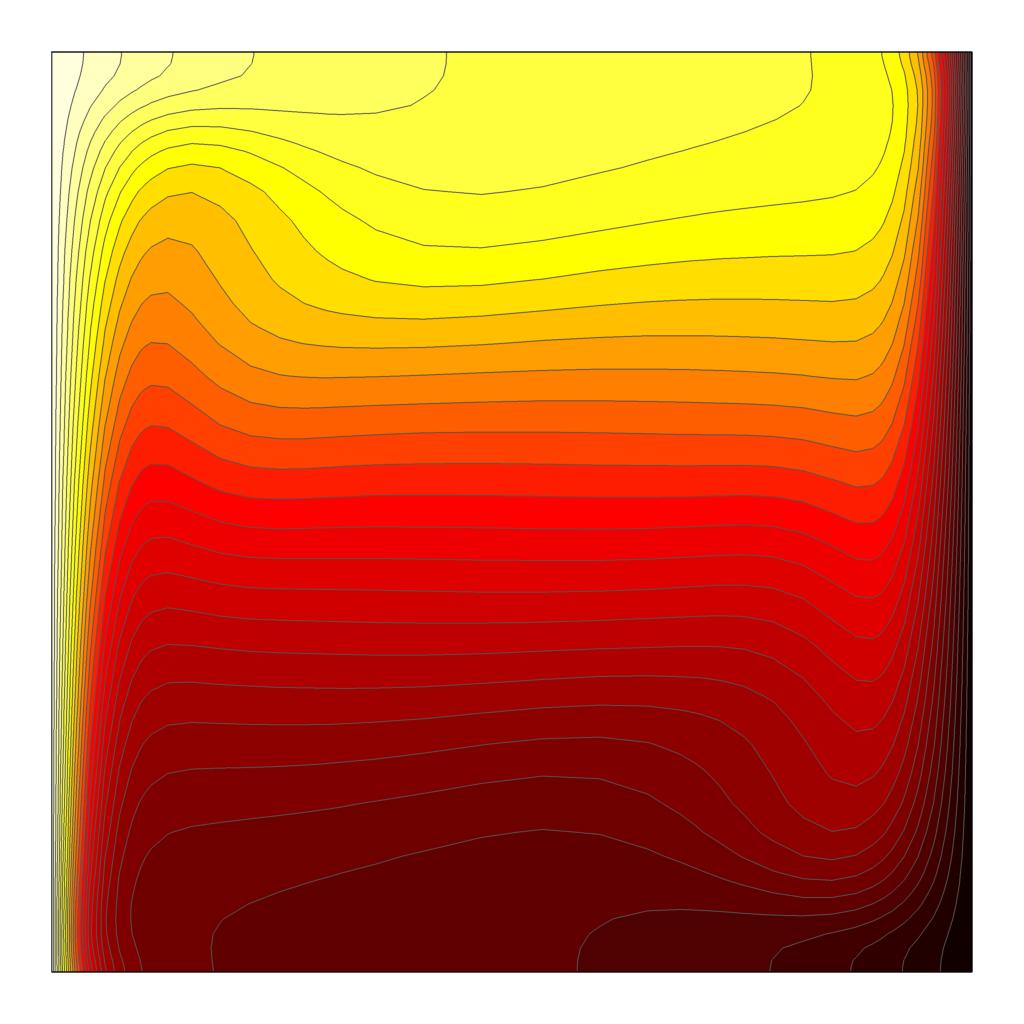  Natural convection in a square cavity at Ra = 10⁶ and Pr = 0.71. Contours of temperature are shown. Top and bottom walls are thermally insulated; left and right walls are fixed hot and cold, respectively.

  This example (download: .tgz or .zip) demonstrates natural convection - a flow driven by buoyancy differences in a fluid. This is achieved through the use of a scalar field representing temperature, and a Boussinesq model for buoyancy coupling the temperature field to the momentum equation. Here the two-dimensional flow in a square cavity filled with air is simulated. The top and bottom walls are thermally insulated, the left wall is hot and the right wall is cold.

  The scalar field is activated by including in the viper.cfg file commands that define aspects of the field. In this case gvar_scalar_diff sets the diffusion coefficient, gvar_init_scalar_field sets the initial value of the field, and two btag statements specify constant Dirichlet conditions on the scalar field for the hot (left) and cold (right) walls.

  The viper.cfg file also demonstrates the use of gvar_usrvar statements to create user-defined functions, here containing constant values of the Rayleigh ("Ra") and Prandtl ("Pr") numbers. These functions can be included in other commands in the viper.cfgfile

  , in macro files, or on the Viper command line.

  The macro file introduces the buoyancy command, used to activate the buoyancy term in the momentum equation, and the flux command, outputting the total temperature flux through each boundary.

  Rayleigh-Bénard convection

  Rayleigh-Bénard convection in an air-filled square cavity at Ra = 10⁸. Red and blue colours indicate hot and cold air, respectively.

  This example (download: .tgz or .zip) demonstrates the emergence of Rayleigh-Bénard convection, where the bottom wall is hot and the top wall cool, creating an unstable stratification of denser air over lighter air. Plumes quickly erupt from the thermal boundary layers on the top and bottom boundaries, before a cavity-scale circulation develops - the "wind of turbulence" - sweeping away the plumes in the process.